BASIC SPECTROSCOPY
Santi Nonell1 and Cristiano Viappiani2
1 Institut Quimic de Sarria
Universitat Ramon Llull
Via Augusta 390, 08017-Barcelona, Spain
santi.nonell@iqs.url.edu
2 Dipartimento di Fisica
Universita degli Studi di Parma
Viale G.P. Usberti 7A, 43100 Parma, Italia
cristiano.viappiani@fis.unipr.it
1. What Is Spectroscopy?
The term "spectroscopy" defines a large number of techniques that use radiation to obtain information on the structure and properties of matter. The basic principle shared by all spectroscopic techniques is to shine a beam of electromagnetic radiation onto a sample, and observe how it responds to such a stimulus. The response is usually recorded as a function of radiation wavelength. A plot of the response as a function of wavelength is referred to as a spectrum.
This chapter gives an overview of the spectroscopic techniques most commonly used in photobiology research. We have restricted ourselves to include only those techniques that use ultraviolet or visible light as the primary stimulus. Also, with the newcomer student in mind, we have chosen to concentrate on describing the principles and main applications of the techniques, keeping the discussions of technical details and the number of equations to a minimum.
2. What Do Photobiologists Use Spectroscopy For?
Photobiologists use a number of spectroscopic techniques to understand how photobiological processes occur. This involves in the first place identifying the primary photoactive molecular entity whose photoexcitation by the absorption of light energy triggers the biological effect. A fundamental property of such entities is their absorption spectrum, which describes their ability to absorb light of different wavelengths. Determining the absorption spectrum of a photoactive agent is the first step in understanding the photobiological process in which it participates.
Equally important is the identification and characterization of all other molecular entities involved in the process: excited states, reactive intermediates, and photoproducts. Spectroscopic techniques are also of great help for this, and even elusive species whose lifetime merely spans a few tens of femtoseconds (1 femtosecond is 10-15 seconds or one billionth of one millionth of a second) can be studied to a high level of detail with spectroscopic tools.
Finally, a sound understanding of photobiological processes requires a complete knowledge of the molecular mechanism through which they operate. The term mechanism refers to the sequence of events that undergo all participating species, the rates at which they occur, and the factors influencing such rates. Time-resolved spectroscopic techniques allow photobiologists to unravel the mechanims of photobiological processes.
This chapter will describe the most common spectroscopic techniques available to the photobiologist, and will illustrate the kind of information that can be gained with these techniques.
3. A General (And Overly Simplified) Photobiology Scheme
Every photobiological process starts with the absorption of light energy by the primary light-absorbing species M that, as a result, is promoted to an electronic excited state M* of higher energy. Molecules in their excited states are metastable species, and eventually return to the ground state giving back the absorbed energy either as light or as heat. In addition, the energy content in ultraviolet and visible radiation is high enough to also promote competing molecular transformations of M* that lead to the formation of reactive intermediates I, and eventually the photoproduct P responsible for the end photobiological effect. The competition between excited-state decay and chemical transformation is an essential feature of all photochemical and photobiological processes, and their relative rates determine the final outcome of the process initiatiated by the absorption of light energy, hence the importance in measuring such rates.
Photobiologists use energy diagrams to visually organize these species, placing them at a height related to their energy (Figure 1). This proves very useful for visualizing the sequence of steps forming the mechanism and the associated energy flows. Spectrocopic techniques help photobiologists determine the energy contents of each participating species and the rate constants of the processes relating them.
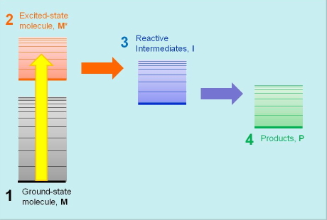
Figure 1. The basic scheme of photobiological events: the primary photoactive molecule M absorbs light and is promoted to its excited state, M*. It then undergoes a chemical transformation to one or more intermediate species I, and finally yields a product P. The vertical position of the bars in the diagram represents the energy content of each species.
4. What Spectroscopies Are Available To The Photobiologist?
Documenting the general photobiological scheme discussed in the previous section requires the identification and characterization of all participating species as well as the determination of the rate constants for the different reactions. Different spectroscopic techniques are available to fulfill this goal, the following being those most commonly encountered in photobiology laboratories.
4.1 Ground-state Absorption
This technique, explained in more detail in Section 5, is applied to stable species, "stable" meaning that their lifetime is at least of a few milliseconds (1 millisecond is one thousandth of a second). This refers tipically to the primary light absorbing agent and the final products. The sample is irradiated with a continuous-wave (CW) beam of light, and the fraction of light absorbed is determined through transmission or reflectance measurements. Because light absorption sends a molecule temporarily to an upper excited state, the information provided by this technique is the absorption spectrum of the photoactive species (Figure 2), the energy difference between their ground- and excited-states, and the probability for light absorption. Absorption transitions are marked with straight arrows on the energy diagram.
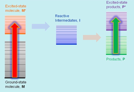
Figure 2. Absorption Transitions In Ground-state Absorption Spectroscopy.
4.2 Transient Absorption
This technique is very similar to the previous one except that the species probed are metastable (i.e., transient) excited states and reaction intermediates whose lifetime may range from femtoseconds, for the primary excited states, to kiloseconds for slow reaction intermediates. The species are promoted temporarily to upper excited states (see Figure 3). Measuring the absorption spectrum of a transient species requires the use of pulsed lasers for generating a measurable concentration of excited states, and a second beam of light, CW or pulsed, for probing their absorption. In addition to absorption spectra, transient absorption techniques also yield the the rate constants of the processes where these species participate.
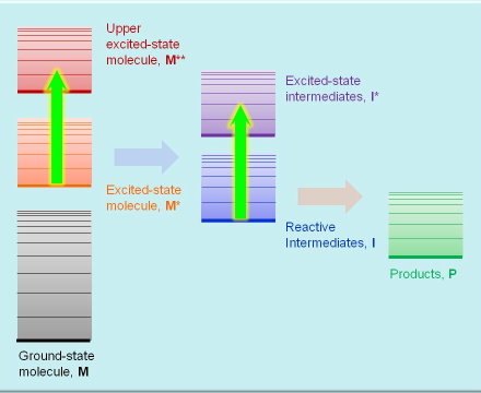
Figure 3. Absorption transitions in transient absorption spectroscopy.
4.3 Emission Techniques
Emission techniques measure the electromagnetic radiation emitted upon deactivation of excited states. When such excited states are created by the absorption of light, the techniques are referred to as fluorescence and phosphorescence, depending on the nature of the excited state. Some chemical and enzymatic reactions also produce excited states, whose emission is then referred to as chemiluminescence. Emission techniques provide emission spectra, excited-state lifetimes, and rate constants for the processes where these species participate. Emission transitions are also signalled by straight arrows on energy diagrams (see Figure 4).
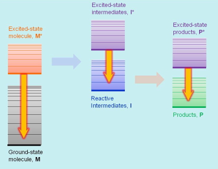
Figure 4. Emission transitions in luminescence spectroscopy.
4.4 Photothermal Techniques
In addition to, and sometimes instead of, emitting light, excited states and reactive intermediates give off their excess energy through non radiative deexcitation pathways, causing local changes in temperature, refractive index and volume. Photothermal techniques monitor such changes and thus provide information on the processes that originate them. The typical use of photothermal techniques is for determining the energy and volume changes accompanying the reactions of the excited states and reactive intermediates (see Figure 5). Thermal or non radiative transitions are conventionally marked with wavy arrows on the energy diagrams.
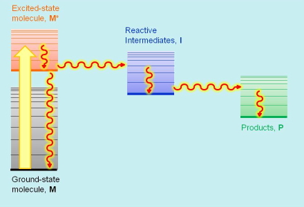
Figure 5. Radiationless transitions in photothermal spectroscopies.
4.5 Time-resolved vs. steady-state techniques.
Optical (absorption and emission) and thermal spectroscopies rely on the creation of excited states and reactive intermediates through the absorption of light, which leads to two fundamentally different approaches: in steady-state spectroscopies the samples are continuosly irradiated with a beam of light; excited states are continuously created and eliminated and eventually a steady-state is reached where their concentration remains constant. This facilitates the measurement of weak signal levels at the expense of loosing kinetic information. Steady-state spectroscopies are best applied to the measurement of absorption and emission spectra. On the other hand, time-resolved spectroscopies rely on the irradiation of the sample with a light source whose intensity fluctuates as a function of time. The simplest example of this is a pulsed laser, which emits flashes of light. Each flash creates a burst of excited states, whose evolution can be monitored as a function of time. Time-resolved spectroscopies provide kinetic information at the expense of a lower sensitivity compared to steady-state techniques.
5. Ground-State Absorption
The absorption spectrum of stable molecules, such as the primary photoactive species or the final products, is most conveniently recorded using a steady-state spectrophotometer. Modern instruments consist of a combination of light sources covering the UV and visible ranges, a monochromator to isolate a narrow wavelength range, a sample compartment, and a detection system (Figure 6). Transparent samples such as films or solutions are best measured in transmission mode, the instrument measuring the intensity of light transmitted by the sample. Opaque or highly scattering samples such as solids or suspensions are best measured in reflectance mode.
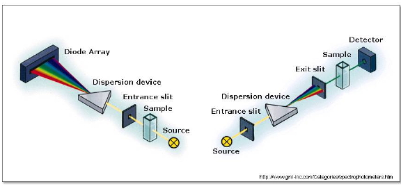
Figure 6. Typical optical layouts for absorption spectrophotometers. Left: In diode-array spectrophotometers, the spectrum is obtained at once. Right: in single detector spectrophotometers, the amount of light transmitted (or reflected) is detected one wavelength at a time.
The transmittance of a transparent sample is defined as the fraction of light transmitted by the sample when it is irradiated with a beam of light. It is determined by measuring the intensity (more properly called radiant power) of the incident and transmitted light beams. A plot of the transmittance vs the beam wavelength is called a transmission spectrum. Photobiologists usually prefer to work with absorption spectra (Figure 7), where the related quantity absorbance is plotted instead. The absorbance of a sample is defined as the negative logarithm of its transmittance: Absorbance = - log (Transmittance). For a pure substance, the absorbance of a sample at a given wavelength is directly proportional to its concentration.
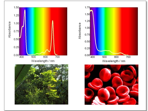
Figure 7. Absorption spectrum of (a) chlorophyll and (b) Fe(II) protoprophyrin IX, the prosthetic group of heme. The sharp absorption of chlorophyll in the red part of the spectrum makes grass green, and its lack in heme makes blood red.
The reflectance of an opaque sample is likewise defined as the fraction of light reflected by the sample when it is irradiated with a beam of light. It is determined by measuring the intensity (radiant power) of the incident and reflected light beams. A plot of the reflectance vs the beam wavelength is called a reflectance spectrum.
Photobiologists use absorption (or reflectance) spectra to: * Identify the wavelengths that a sample can absorb and the relative probabilities of the absorption transitions at each wavelength.
* Identify the molecular species responsible for the photobiological effect under study.
* Determine the energy of the molecule's excited states.
* Study the interactions between species, e.g., a drug with a host protein.
6. Transient Absorption
6.1 The pump-and-probe approach
Transient absorption techniques rely on the use of a probe beam that interrogates the sample before and after excitation with a pulsed laser (pump beam), and monitors absorbance changes either at a selected wavelength (kinetics) or simultaneously at several wavelengths (transient spectra). These methods are collectively referred to as pump-and-probe methods although, depending on the time scale, the transient absorbance techniques may have very different experimental layouts. These techniques allow, in general, to study the disappearance of the excited state M*, the formation of the reactive intermediates I, and the formation of photoproducts P.
The pump laser must excite the sample at a wavelength where ground state absorption occurs (Section 5). The laser pulse width must be much shorter than the time constant of the reaction under investigation.
The probe beam is generally a broadband light source in the UV-vis-NIR spectral range, where transient electronic transitions occur. The probe light source is normally a CW or pulsed lamp for nanoseconds (1 nanosecond is one billionth of a second) or longer time scales, while a pulsed laser is used for higher time resolution.
The experimental parameter of interest is a change in sample absorbance (
 A), obtained from the change in transmitted light intensity of the probe beam before, I(t<to), and after, I(t), laser excitation, according to the following equation:A(t)= -log [I(t)/I(t<to)].
Photobiologists use transient absorption to:
* Identify reaction intermediates from their spectral features
* Assess the reaction mechanism by detecting spectrally distinguishable reaction intermediates
* Determine the rate constants for each kinetic step
* Determine activation parameters from temperature dependence of rate constants
* Determine reaction quantum yields in favourable cases, where extinction coefficients of reaction intermediates are known.
6.2 From milliseconds to hours: steady-state spectrophotometers
When very slow reactions (time constants in the range of minutes or longer) are to be monitored, the changes in the absorbance of the sample following photo-excitation by the pulsed laser can be followed using conventional steady state spectrophotometers (Section 5), provided that the absorption spectra can be taken on time scales much faster than the characteristic time of the reaction under investigation. Spectrophotometers also allow one to follow the absorbance at a selected wavelength as a function of time, thus providing a kinetic time course for the photoinduced reaction.
For faster reactions (down to a few milliseconds) multichannel detectors, such as charge coupled devices (CCDS), and photodiode arrays (PDA) are normally used to follow the time evolution of the absorption spectrum. In these applications, a CW broadband light source is used to probe the absorption of the sample. The polychromatic beam is passed through a spectrograph to measure absorption spectra as a function of time. (Figure 6, left) Specialized setups also allow to follow the absorbance at a selected wavelength as a function of time.
6.3 From milliseconds to nanoseconds: nanosecond laser flash photolysis
Absorbance changes, from milliseconds to nanoseconds, following excitation with a nanosecond pulsed laser can be monitored using a CW light source such as a Xe arc lamp (Figure 8). A fast shutter exposes the sample to the probe beam shortly before the laser pulse hits the sample, and is closed after the end of data collection to prevent its photobleaching. (Figure 9) The polychromatic beam is passed through a spectrograph, either to select the wavelength at which the reaction kinetics are monitored or to measure transient spectra as a function of time (Figure 10). Examples of time-resolved spectra and rebinding kinetics are displayed in Figures 11 and 12. The spectral and kinetic information allow to identify reaction intermediates and to retrieve rate constants.
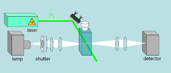
Figure 8. Essential optical layout of a nanosecond laser flash photolysis setup. A CW lamp beam monitors changes of absorbance (or reflectance) in a sample after flash photoexcitation with a pulsed laser.
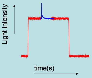
Figure 9. Time profile of probe light intensity transmitted by the sample. At time zero, the shutter is closed and the detector sees no light. When the shutter is opened the light transmitted by the sample is seen by the detector. The changes in intensity induced by the pulsed laser are highlighted as a blue signal. At the end of the experiment the shutter is closed again to prevent extensive photodegradation of the sample.
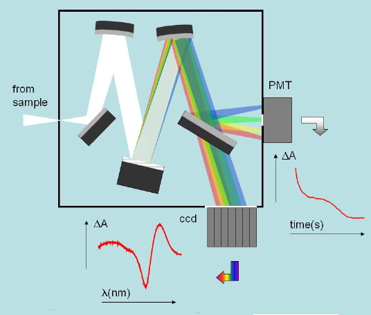
Figure 10. Typical optical layout of the detectors used in nansoecond laser flash photolysis. The spectrograph can select a specific wavelength and allow monitoring the absorbance changes at that wavelength. Alternatively, a spectral range can be monitored by a multichannel detector such as a (CCD) and allow the determination of transient spectra at selected time delays.
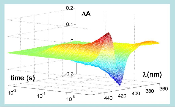
Figure 11. Time-resolved changes in absorption spectrum following photodissociation of carboxy-hemoglobin. A nanosecond laser pulse photolyzes the CO-Fe bond leading to changes in the heme absorption spectrum in the Soret region. The ligand is then rebound by the heme, with the complex kinetics shown in the plot, extending over several orders of magnitude in time. The protein is embedded in a silica gel to prevent quaternary switching from the R to the T quaternary structure after photodissociation.
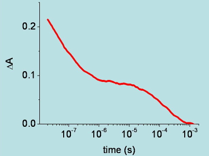
Figure 12. Time course of the change in absorbance at 436 nm, following nanosecond photodissociation of carboxy-hemoglobin. The change in absorbance reflects the kinetics of carbon monoxide rebinding to the heme Fe.(see Viappiani, C. et al. Proc. Natl. Acad. Sci. USA 2004, 101, 14414-14419. for details).
6.4 The subnanosecond domain: the two-pulse pump-and-probe technique
When absorbance changes are to be monitored in the subnanosecond domain, the probe beam is obtained by a second broadband laser pulse, hitting the photoexcited sample at a proper time delay (Figure 13).
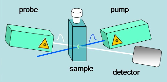
Figure 13. Scheme for sub-nanosecond pump-and-probe methods.
Modern pump lasers emit pulses of approx. 100 femtoseconds, which are tuneable across broad wavelength ranges, and have a high repetition rate (80 MHz). The probe beam is normally obtained by splitting a portion of the pump beam, which is then focussed onto suitable materials generating spectrally broad pulses in the region of interest. Kinetic information is obtained by adjusting the time delay between pump and probe pulses. By probing the photoexcited sample as a function of time delay of the probe pulses, time-resolved spectra can be obtained, from which the kinetics at selected wavelengths can be reconstructed. Results are similar to those represented in Figures 11 and 12, except for the time scale.
7. Emission Spectroscopies
In emission spectroscopy, a sample is irradiated with a beam of light (the excitation beam), and the luminescence emerging from the cuvette is recorded with a suitable detector. Such luminescence is caused by the radiative decay of the excited states created by the excitation beam, which thereby return to their ground state. The emission detector is placed tipically at right angle to the excitation beam to avoid any transmitted light. (Figure 14).
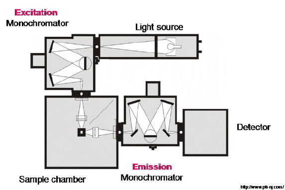
Figure 14. Optical layout of a steady-state spectrofluorometer. A light beam produced by a CW lamp is passed through a monochromator to select a particular excitation wavelength that is then focused onto a sample. The ensuing emission is observed at right angles, analyzed spectrally with the emission monochromator, and recorded by an appropriate detector.
When the excited state has the same spin multiplicity as the ground state the radiative decay transition is labelled as "spin allowed" and the emission is referred to as fluorescence. When the spin changes the transition is said to be forbidden and the emission is called phosphorescence. From a kinetic point of view, fluorescence emission is a fast process, typically in the nanosecond range, while phosphorescence may last anything from microseconds to hours. In addition, phosphorescence always occurs at longer wavelengths than fluorescence (Figure 15).
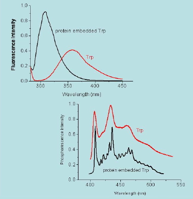
Figure 15. Fluorescence (top) and phosphorescence (bottom) spectra of tryptophan in a protein (black) and in solution (red). Notice that phosphorescence occurs at longer wavelengths than fluorescence. Data are courtesy of P. Cioni, CNR, Pisa (Italy).
7.1 Steady-state emission spectroscopy
In steady-state spectrofluorometers, the sample is irradiated with a CW beam of light, very much as in absorption spectroscopy. This creates a steady concentration of excited states, and therefore a steady emission of light from the sample. Excitation and emission monochromators allow the user to select the wavelengths of the excitation and emission beams.
Emission spectra are obtained by setting the excitation wavelength to a constant value and scanning the emission monochromator. The recorded emission intensity is then plotted as a function of the emission wavelength (Figure 16). Alternatively, the emission wavelength is locked and the excitation monochromator is then swept. This produces an excitation spectrum. For a pure substance existing in a single molecular form in the sample the excitation spectrum matches its absorption spectrum, which is very useful to identify the emitting species in a mixture. Differences between absorption and excitation spectra indicate the presence of more than one species in the sample, either due to different substances or different forms of the same substance, e.g. an acid and its conjugated base or a monomer and a dimer, etc.
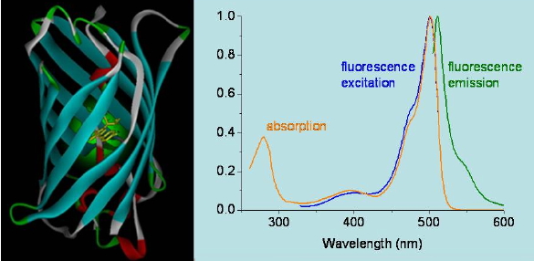
Figure 16. Absorption, fluorescence emission, and fluorescence excitation spectra of a green fluorescence protein mutant.
The fluorescence (or phosphorescence) quantum yield expresses the probability of emitting light upon absorption of radiation and is calculated by dividing the number of light quanta emitted by the number of quanta absorbed.
Photobiologists use steady-state emission spectroscopy to:
* Assess the ability of a substance to emit light, and the wavelengths where this emission occurs. The corresponding properties are the emission quantum yield and the emission spectrum.
* Identify the molecular species responsible for the photobiological effect under study. This is inferred from the excitation spectrum.
* Determine the energy of the molecule's excited states. The wavelength of the fluorescence onset gives a good estimation of the energy of the first excited singlet state, while that of the phosphorescence onset gives the energy of the triplet state.
* Study the interactions between species, e.g., a drug with a host protein, which often result in changes of the spectrum and/or quantum yield of the emission.
7.2 Time-resolved emission spectroscopy
Time-resolved emission spectroscopy provides information on the kinetic behavior of luminescent excited states and intermediates. The optical layout is essentially identical to that given in Figure 14, but a light source whose intensity changes as a function of time is used instead. This creates a population of luminescent species that also change over time and therefore renders it possible to monitor the emission decay kinetics (Figure 17). Typical light sources include pulsed or modulated lamps, light-emitting-diodes, or lasers.
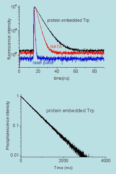
Figure 17. Decay of fluorescence (top) and phosphorescence (bottom) of tryptophan in a protein (black) and in solution (red; actually the sample is N-acetyl-tryptophan-amide, NATA). Notice that phosphorescence lasts much longer than fluorescence. Data are courtesy of P. Cioni, CNR, Pisa (Italy) and T. Gensch, Research Center Jülich (Germany).
Photobiologists use time-resolved emission spectroscopy to:
* Obtain rate constants for processes involving luminescent species. These are in most cases obtained in a straightforward way from the kinetic analysis of the intensity-vs-time luminescence data.
* Unravel the mechanism of a photobiological process by characterizing the reactive intermediates and their rates of formation and decay. This is usually achieved from the analysis of time-resolved emission spectra (TRES), where the luminescence is recorded both as a function of time and wavelength.
* Study the interactions between species, e.g., a drug with a host protein. This is particularly useful when such interactions have no measurable effect on the emission spectra of host or guest but rather on their luminescence lifetimes.
8. Photothermal Techniques
Photothermal tecniques are a group of high sensitivity methods that monitor the effects induced in solution after non-radiative relaxation of excited states. The basis of the collective term photothermal for these techniques lays in the detection of thermal relaxation of excess energy associated with photo-excitation of the sample. In addition, other non-radiative non-thermal relaxations, such as volumetric changes due to photoinduced structural changes (isomerization, charge transfer, solute-solvent rearrangement, ...) may give rise to detectable signals. The most remarkable advantage of these methods is that, through a proper analysis, thermodynamic parameters (energy and volume changes) for each step of the photoinduced reaction can be obtained. The inherent time resolution of the methods allows one to also retrieve kinetic parameters (rate constants, quantum yields) for the reaction steps. Time-resolved photoacoustics is the technique of choice for reactions steps with lifetimes between about 10 nanoseconds and 10 microseconds. For photoinduced reactions with longer time constants, photorefractive methods are more adequate, since they can access events with lifetimes extending to the milliseconds.
Photothermal methods generally apply to optically transparent, low absorbing samples, although time-resolved photoacoustics can be applied to strongly absorbing samples, with dedicated experimental setups.
Photobiologists use photothermal methods to:
* Estimate enthalpy and volume changes for each kinetic step
* Estimate the energy content of reaction intermediates
* Determine the quantum yield of photo-initiated reactions
* Determine the rate constants for each kinetic step
8.1 Time-resolved photoacoustics
Time-resolved photoacoustics monitors the pressure changes induced in a sample after non-radiative relaxations following excitation with a (normally) nanosecond pulsed laser. The pressure pulse generally has two sources, both leading to a volume change of the solution, and related with non-radiative relaxations of the excited state. The first source is the thermal relaxation associated with energy changes accompanying relaxation of the excited state and reaction intermediates. The second source is due to volume changes associated with structural rearrangements accompanying each step of the photoinduced reaction. The time evolution of the pressure pulse is monitored in microseconds (one microsecond is one millionth of a second) by a fast piezoelectric microphone (Figure 18). Calibration of the setup to retrieve thermodynamic and kinetic parameters implies comparison of the photoacoustic signal with that obtained for a photocalorimetric reference compound (i.e., a compound that undergoes thermal relaxation with unit efficiency within a few nanoseconds). (Figure 19) The resonant configuration of the detector requires the use of numerical deconvolution analysis to retrieve kinetic information from experimental signals.
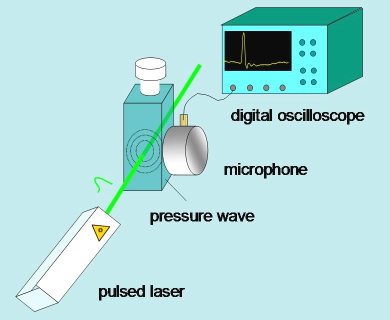
Figure 18. Essential scheme of a time resolved photoacoustics setup.
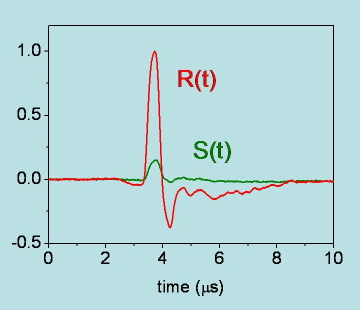
Figure 19. Photoacoustic signals for degassed acetonitrile solutions of the photocalorimetric reference compound 2,hydroxybenzophenone (R(t)) and benzophenone (S(t)) at room temperature. Both the amplitude and the shape of the signal for benzophenone are different from those for 2,hydroxybenzophenone. The signal for benzophenone, of thermal origin, is best described by a double exponential decay with a fast component (lifetime below ( 10 ns), due to triplet formation, and a slower relaxation (lifetime of ( 6.7 microseconds), due to triplet decay.
8.2 Photorefractive techniques
Photothermal lensing, beam deflection, and grating techniques detect changes in refractive index upon changes in density (resulting from a change in volume of either thermal of structural origin), in absorbance, and in temperature. When a sample is excited with a light beam, which usually has a Gaussian shape, being absorbed by the sample, the concentration of the excited state molecules reflects the pump beam geometry. The non-radiative relaxations of the excited states heat the sample resulting in a temperature profile, which reflects the Gaussian intensity profile of the exciting laser beam. A decrease in density results from heating, eventually leading to a decrease in the refractive index of the sample. These methods allow one to retrieve enthalpy and volume changes associated with the relaxation of the photexcited molecules, and the rate constants of these processes.
Three basic experimental approaches are used to detect the refractive index change: the transient lens, the beam deflection, and the transient grating.
Transient lens. A CW probe beam travels through the illuminated region (by the pump laser) and is expanded by the Gaussian profile of the refractive index. This effect can be detected from the change in light intensity through a pinhole (Figure 20).
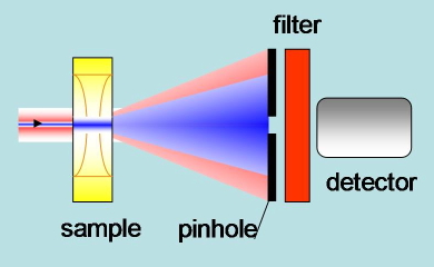
Figure 20. Schematic of the experimental setup in transient lens experiments. The pump blue beam generates a change in refractive index. The red probe beam is expanded by the refractive index profile. A detector placed after a pin hole senses the defocusing as a change in light intensity.
Beam Deflection. The CW probe beam is not perfectly concentric with the pump beam. The spatial profile of the refractive index change results in a deflection of the probe beam. A position sensitive detector monitors the displacement of the probe beam (Figure 21).
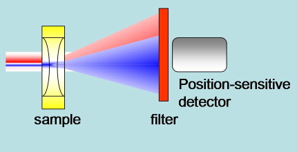
Figure 21. Schematic of the experimental setup in beam deflection experiments. The pump blue beam generates a change in refractive index. The red probe beam is deflected by the refractive index profile. A position sensitive detector senses the deflection.
Transient Grating. Two pump laser beams with parallel polarization are brought into the sample at an angle and from their interference pattern a modulation of the excitation intensity results. The refractive index changes originating from the photoinduced processes reflect this modulation, and can be monitored by a third laser beam, which is diffracted to an extent depending on the grating properties. An advantage of this method is that it can access subnanosecond events (Figure 22).
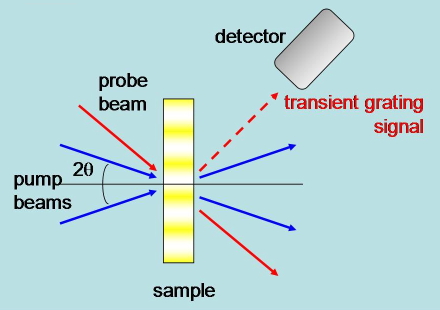
Figure 22. Schematic of the experimental setup in transient grating experiments.
The rate of formation of the density lens (≈ 107 s-1) sets the time resolution in transient lens and beam deflection. On the other hand, the techniques are very sensitive in detecting slower kinetics, extending to milliseconds. In order to retrieve quantitative thermodynamic information from the lens and beam deflection signals, a photocalorimetric reference must be used to calibrate the instrumental response, in essentially the same way as already described for the photoacoustic signals. The advantage of these methods is that they require no deconvolution analysis to retrieve the kinetic information.
9. Concluding Remarks
The photobiologist of the 21st century might rather be called a molecular photobiologist in that the molecular approach provides the most accurate albeit complex description of photobiological phenomena. Spectroscopy offers a wonderful window into such a molecular world, and provides us with a unique yet powerful set of tools to explore the intricacies of photobiological phenomena. Techniques that were rather sophisticated just a decade ago are now being routinely used in many laboratories worldwide, revealing a wealth of data which is changing the way we understand nature.
10. Further Reading
Nanosecond Laser Flash Photolysis
Bonneau R., Wirz J., Zuberbuehler A.D. (1997) Methods for the analysis of transient absorbance data, Pure & Appl. Chem. 1997, 69, 979-992.
Chen E., Goldberg R. A., Kliger D.S. Nanosecond time-resolved spectroscopy of biomolecular processes, Ann. Rev. Biophys. Biomol. Struct. 26, 327-355.
Tetreau C., Lavalette D. (2005) Dominant features of protein reaction dynamics: Conformational relaxation and ligand migration, Biochim. Biophys. Acta 1724, 411-424.
Abbruzzetti S., Bruno S., Faggiano S., Grandi E., Mozzarelli, A., Viappiani, C. (2006) Time-resolved methods in Biophysics. 2. Monitoring haem proteins at work with nanosecond laser flash photolysis, Photochem. Photobiol. Sci., 5, 1109-1120.
Picosecond Transient Absorbance
Cerullo, G., Manzoni C., Luer L., Polli, D. (2007) Time-resolved methods in biophysics. 4. Broadband pump-probe spectroscopy system with sub-20 fs temporal resolution for the study of energy transfer processes in photosynthesis, Photochem. Photobiol. Sci., 6, 135-144.
Groot, M.L., van Wilderen, L.J.G.W., Di Donato, M. (2007) Time-resolved methods in biophysics. 5. Femtosecond time-resolved and dispersed infrared spectroscopy on proteins, Photochem. Photobiol. Sci., 6, 501-507.
Emission Spectroscopy
Lakowicz, J.R. (2006) Principles of Fluorescence Spectroscopy, 3rd ed., Kluwer Academic/Plenum Publishers, New York.
Becker, W. (2005), Advanced Time-Correlated Single Photon Counting Techniques, Springer, Germany.
Time Resolved Photoacustics
Braslavsky, S.E., Heibel, G.E. (1992) Time-resolved photothermal and photoacoustics methods applied to photoinduced processes in solution, Chem. Rev. 92, 1381-1410.
Gensch, T., Viappiani, C. (2003) Time-resolved photothermal methods: accessing time-resolved thermodynamics of photoinduced processes in chemistry and biology, Photochem. Photobiol. Sci. 2, 699-721.
Photorefractive Techniques
Schulenberg, P. J.; Braslavsky, S. E. (1997) Time-resolved photothermal studies with biological supramolecular systems, in Progress in Photothermal and Photoacoustic Science and Technology, Mandelis, A., Hess, P., Eds, SPIE Optical Engineering Press, Washington, pp. 57-81.
Terazima, M. (2001) Protein dynamics detected by the time-resolved transient grating technique, Pure & Appl. Chem. 73, 513-517.
10/16/08